# tossing a fair coin once
rbinom(1, 1, 0.5)
[1] 1This reading guide is a reconstructed Quarto .qmd file made from the HTML you provided.
It is a best-effort skeleton: headings, math, text snippets, and the interactive R code chunks that were embedded in the HTML (extracted from the page’s webR cell definitions).
Some layout, styling, and Quarto-specific extensions from the original site (webR integration, Monaco editor options, custom CSS/JS, and ancillary assets) are not reproduced here. Use quarto render to generate HTML and the _files folder.
(Original text omitted for brevity — paste in more content from the HTML if you want the full text.)
(From Evans and Rosenthal) Suppose \(S=\{1,2,3\}\) and we try to define \(\mathbb{P}\) by the following rules:
Suppose Ronald and Robert are students in a statistics course. Define \(A\) as the event Ronald passes the course and \(B\) as the event Robert passes the course. Suppose \(\mathbb{P}(A)=0.9\) and \(\mathbb{P}(B)=0.7\). What is the probability that both pass the course if
Consider the sample space \(S=\{0,1\}\). Let \(p\in(0,1)\). Let \(\mathbb{P}\) be a probability function where \(\mathbb{P}(\{1\})=p\) and \(\mathbb{P}(\{0\})=1-p\).
Below are the R code cells that were embedded in the original HTML (extracted from the webR cell definitions). They are included as typical Quarto R code blocks.
# tossing a fair coin once
rbinom(1, 1, 0.5)[1] 1# what does this do?
rbinom(10, 1, 0.5) [1] 1 0 1 0 0 0 1 1 0 1# what is the point of this?
x <- rbinom(10, 1, 0.5)x [1] 0 1 1 0 0 1 1 1 0 1length(x)[1] 10c(1, 3, 8)[1] 1 3 8cumsum(c(1, 3, 8))[1] 1 4 12c(1, 3, 8)/3[1] 0.3333333 1.0000000 2.66666671:20 [1] 1 2 3 4 5 6 7 8 9 10 11 12 13 14 15 16 17 18 19 20c(1, 3, 8)/(1:3)[1] 1.000000 1.500000 2.666667c(1:3, 5:7)[1] 1 2 3 5 6 7c(1,3,8)/c(2,3) # be careful here.Warning in c(1, 3, 8)/c(2, 3): longer object length is not a multiple of
shorter object length[1] 0.5 1.0 4.0rep(1:3, 10) [1] 1 2 3 1 2 3 1 2 3 1 2 3 1 2 3 1 2 3 1 2 3 1 2 3 1 2 3 1 2 3z <- cumsum(x)/(1:length(x))
z [1] 0.0000000 0.5000000 0.6666667 0.5000000 0.4000000 0.5000000 0.5714286
[8] 0.6250000 0.5555556 0.6000000plot(z)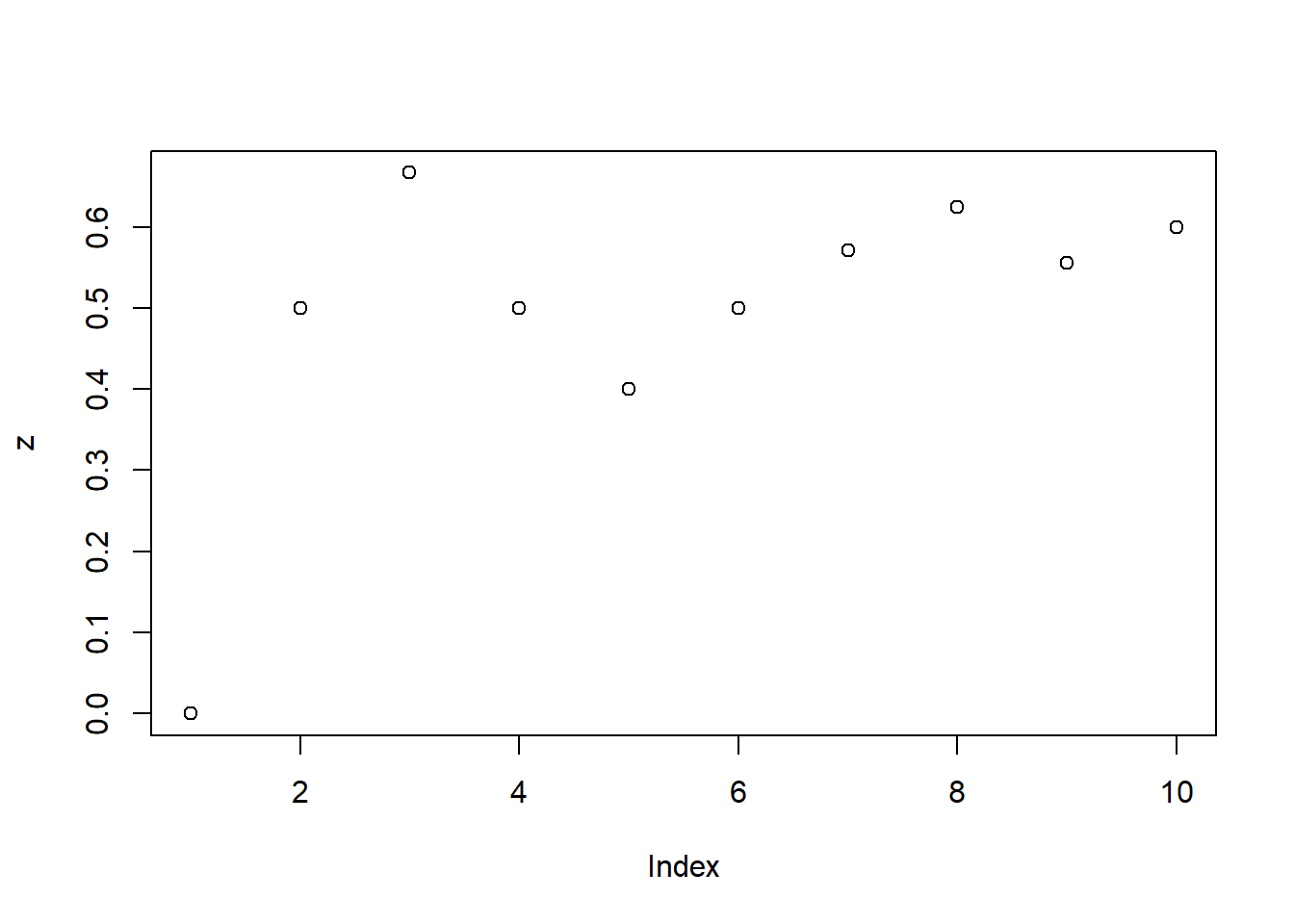
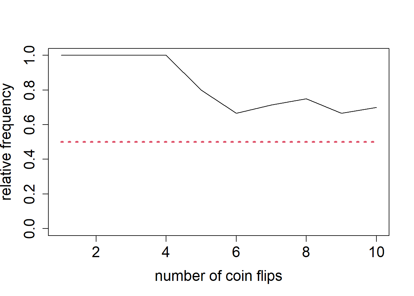
plot(1:length(z),
     z,
     type = "l",
     xlab = "number of coin flips",
     ylab = "relative frequency",
     ylim = c(0, 1),
     cex.lab = 1.5,
     cex.axis = 1.5)
lines(1:length(z),
      rep(0.5, length(z)),
      lty = 3,
      col = 2,
      lwd = 3)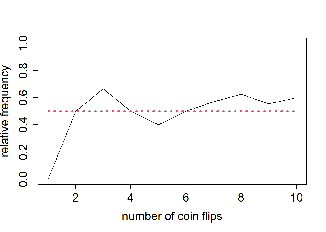
x <- rbinom(10, 1, 0.5)
z <- cumsum(x)/(1:length(x))
plot(1:length(z), z, type = "l", xlab = "number of coin flips", ylab = "relative frequency", ylim = c(0, 1), cex.lab = 1.5, cex.axis = 1.5)
lines(1:length(z), rep(0.5, length(z)), lty = 3, col = 2, lwd = 3)